Prototyping a demo Web Application for ML Models, Technilog

• 1: Implementation of the Web Application
• 2: Models used
• 3: Work Completed
• 3.1: Forecast Simulation
• 3.2: System Anomaly Detection
• 3.3: Impact Study
• 3.4: Update, QOL ("Qualities Of Life")

About Technilog

Technilog is a service company specializing in the development of software solutions for the integration of connected industrial objects or IIOT (“Industrial Internet of Things”). Technilog offers two flagship software solutions: Dev I/O, a remote management and supervision software that unifies and processes data from connected equipment, and Web I/O, a platform for the supervision and control of connected objects across various platforms.

Source: Technilog

Context

As part of the evolution of IoT solutions offered by Technilog, a new version of their flagship product, Web I/O, has been developed. This version integrates advanced features, including artificial intelligence (AI) tools. To illustrate these tools, a web application was created to demonstrate the use cases and capabilities of this new version.

Achievements

An initial version of this demonstration site was developed by the previous intern. In this version, data qualification functionalities and variable anomaly detection were implemented. Additionally, the necessary infrastructure for web hosting of the application was set up. My role was to add new features and participate in the design meetings for the web pages:

• Anomaly Detection: Based on machine learning from historical data, this feature determines if a value behaves unusually.
• Forecast Simulation: Similar to anomaly detection, this feature uses machine learning from historical data. From this learning and previously obtained values, a model can be determined to anticipate future values.
• Impact Study: Allows evaluating the impact that different variables have on each other, as well as the relationships between these variables, providing an in-depth understanding of the mutual influences of these components.
• Quality of Life Improvements: Addition of authentication features and model updates.
• Deepening Knowledge: In-depth study of various artificial intelligence models.

1 - Implementation of the Web Application

Introduction to Dash

Dash is a Python framework for creating interactive web applications. It operates with layouts and callbacks. In our implementation, we also use the Plotly library for data visualization and graphs.

Source: Plotly

Functionality

The framework operates with layouts and callbacks, these components define the appearance and functionality of the application.

Layouts

Layouts define the appearance of the application. They consist of standard HTML elements or interactive components from specific modules. A layout is structured as a hierarchical tree of components, allowing for the nesting of elements.

Dash is declarative, meaning that all components have arguments that describe them. The arguments can vary depending on the type of component. The main types are HTML components (dash.html) and Dash components (dash.dcc).

The available HTML components include all standard HTML elements, with attributes such as style, class, id, etc. Dash components generate high-level elements such as graphs and selectors.

Callbacks

Callbacks are functions automatically called when an input component (input) changes. They display the result of the functions to an output component (output).

Callbacks use the @callback decorator to specify the inputs and outputs, corresponding to the id of the components and the properties to be updated. Each attribute of a component can be modified as an output of a callback, in response to an interaction with an input component. Some components, like sliders or dropdowns, are already interactive and can be used directly as inputs.

Example Code

Here is an example of code illustrating the use of Dash and Plotly: Documentation

from dash import Dash, html, dcc, callback, Output, Input
import plotly.express as px
import pandas as pd

# Loading data
df = pd.read_csv('https://raw.githubusercontent.com/plotly/datasets/master/gapminder_unfiltered.csv')

# Initializing the Dash application
app = Dash()

# Defining the application layout
app.layout = html.Div([
    html.H1(children='Title of Dash App', style={'textAlign':'center'}),
    dcc.Dropdown(df.country.unique(), 'Canada', id='dropdown-selection'),
    dcc.Graph(id='graph-content')
])

# Defining the callback to update the graph
@callback(
    Output('graph-content', 'figure'),
    Input('dropdown-selection', 'value')
)
def update_graph(value):
    # Filtering data based on the country selection
    dff = df[df.country == value]
    # Creating a line graph with Plotly Express
    return px.line(dff, x='year', y='pop')

# Running the application
if __name__ == '__main__':
    app.run(debug=True)

2 - Models used

The Machine Learning and Deep Learning models used for the implemented features include time series forecasting models and autoencoder models.

Time Series Forecasting

Source : Lightning AI

Time series forecasting models allow for predicting future values over a given period. They are developed from historical data to predict future values.

A time series is a set of data points ordered in time, such as temperature measurements taken every hour during a day.

The predicted values are based on the analysis of past values and trends, assuming that future trends will be similar to historical trends. It is therefore crucial to examine trends in historical data.

The models make predictions based on a window of consecutive samples. The main features of the input windows include the number of hourly points and their labels, as well as the time offset between them. For example, to predict the next 24 hours, one can use 24 hours of historical data (24 points for windows with an hourly interval).

Auto-encoder

Source : IBM

Autoencoder models are neural networks designed to copy their input to their output. They first encode the input data into a lower-dimensional latent representation, then decode this representation to reconstruct the data. This process allows for compressing the data while minimizing the reconstruction error.

In our case, these models are trained to detect anomalies in the data. Trained on normal cases, they exhibit a higher reconstruction error when faced with abnormal data. To detect anomalies, it is sufficient to set a reconstruction error threshold.

Conclusions

These models play a crucial role in the project by enabling accurate predictions and anomaly detection. Although I did not directly participate in their development, this internship offered me a valuable opportunity to deepen my knowledge of machine learning and understand the importance of these models in real-world applications. These tools not only help anticipate future trends but also identify unusual behaviors, contributing to more informed and proactive decision-making, which is relevant for IoT.

3 - Work Completed

Achievements

As indicated on the summary page, an initial version of the site had already been implemented by the previous intern. In this version, the data qualification and variable anomaly detection features were put in place. Additionally, the infrastructure necessary for web hosting of the application was installed. This infrastructure is hosted on OVHCloud, using an Ubuntu 22.04 distribution, and the application is deployed with Flask.

For this internship, the missing features will need to be implemented, including forecast simulation, systemic anomaly detection, and impact study. Additionally, quality of life (QOL) improvements will be made.

3.1 - Forecast Simulation

The implementation of the forecasting feature was done in the same manner as the other functionalities: creating the layout, defining the callbacks, and setting up the associated container. This approach was applied to all new features.

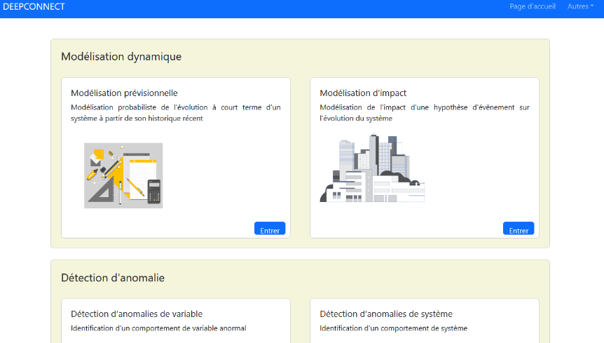
This feature aims to present the different models available for predicting variables such as temperature, pressure, power, etc. The models are trained on data from Technilog sensors, clients, or artificial sources. The feature includes two tabs:

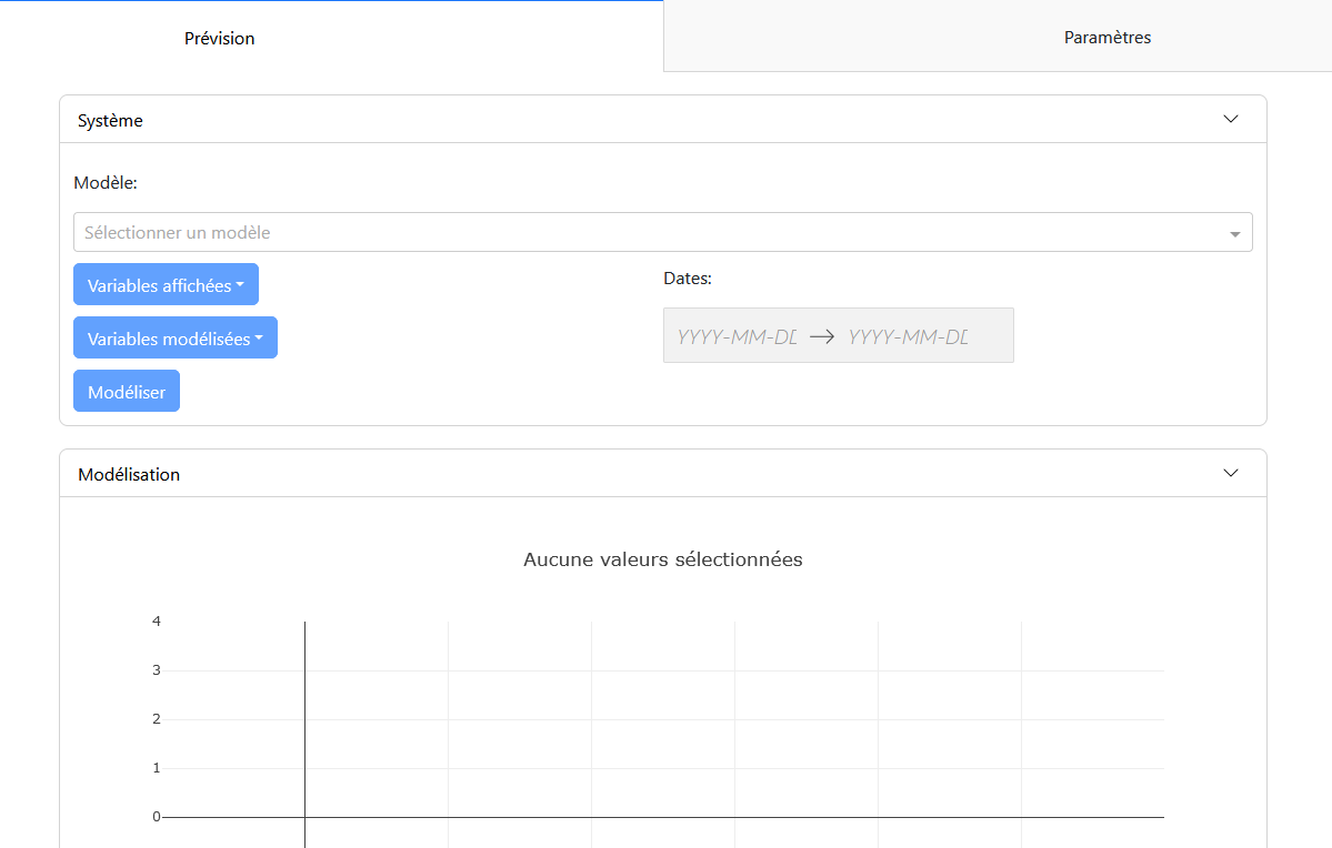
• Forecast Tab: This tab contains the configuration panel “System” and the modeling panel “Modeling.”
• Configuration Panel: Allows for selecting the modeling parameters, such as the model, input variables, variables to display, variables to model, and the study period. Once the variables are selected, it is possible to perform the prediction and visualize the modeling.
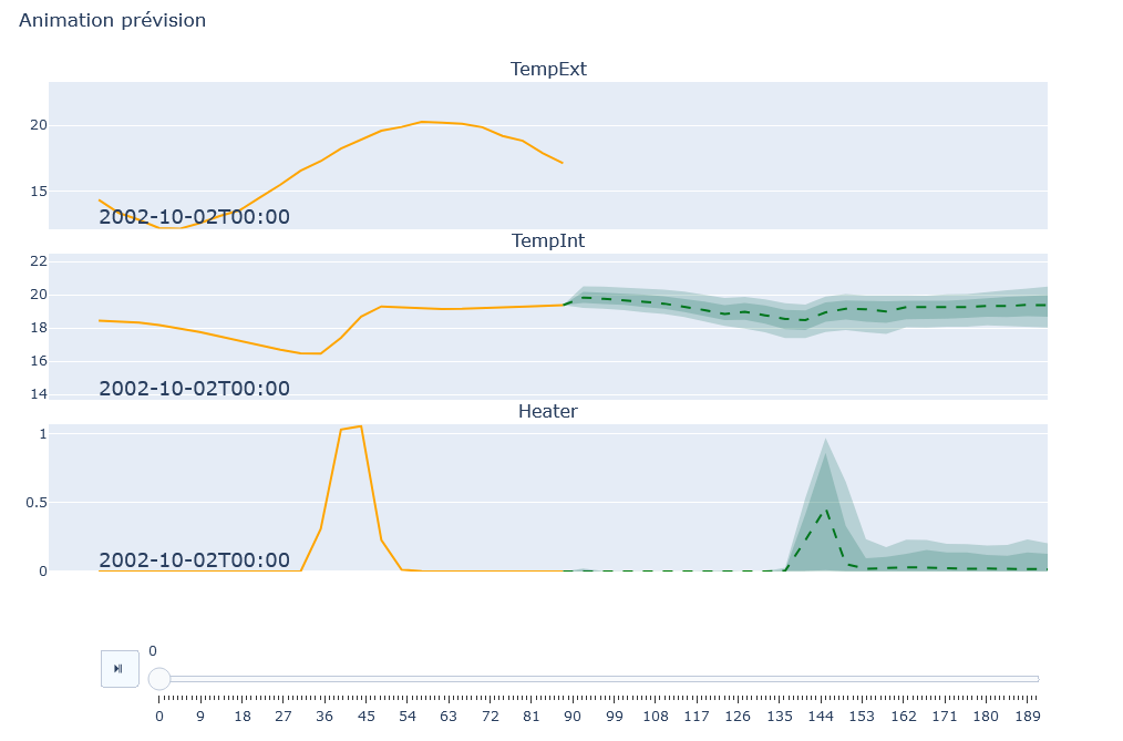
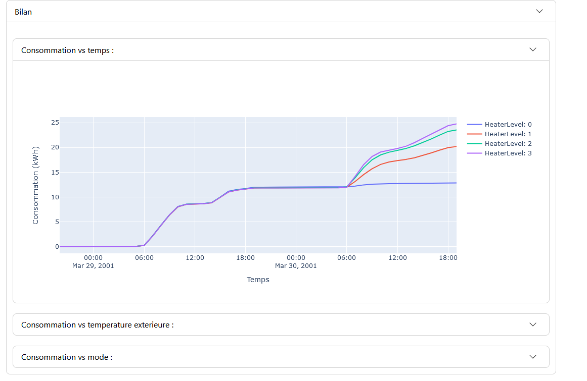
• Modeling Panel: Displays the modeling graphs for each variable. The graphs show the actual data in orange and the predictions with uncertainty in green. Control buttons allow managing the animation, if this option is enabled.

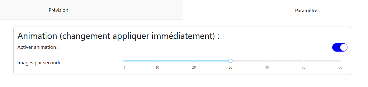
• Settings Tab: Contains the parameters for the modeling animation, such as enabling the animation and the number of frames per second. These options are saved and applied to all models in the feature.

3.2 - System Anomaly Detection

For system anomaly detection, three tabs are available: “Real-time,” “Historical,” and “Settings.” The “Real-time” and “Historical” tabs correspond to different use cases of the feature.

“Real-time” Tab

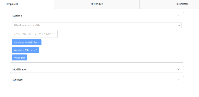
In the “Real-time” tab, you will find the configuration panels “System,” modeling “Modeling,” and summary “Summary.”

• Configuration Panel: Allows you to select the model, modeled variables (variables monitored to determine anomalies), displayed variables (variables visible in the modeling panel), and the measurement period (start and end dates). Default values exist depending on the selected model.

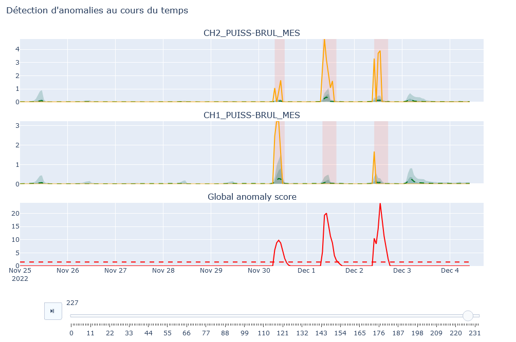
• Modeling Panel: Displays graphs of the selected values with their models. If the anomaly threshold is enabled in the “Settings” tab, a graph of the anomaly score is also displayed, highlighting areas where the score exceeds the threshold.

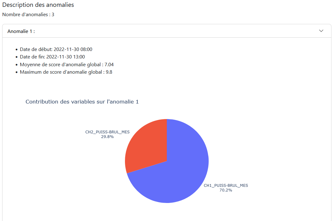
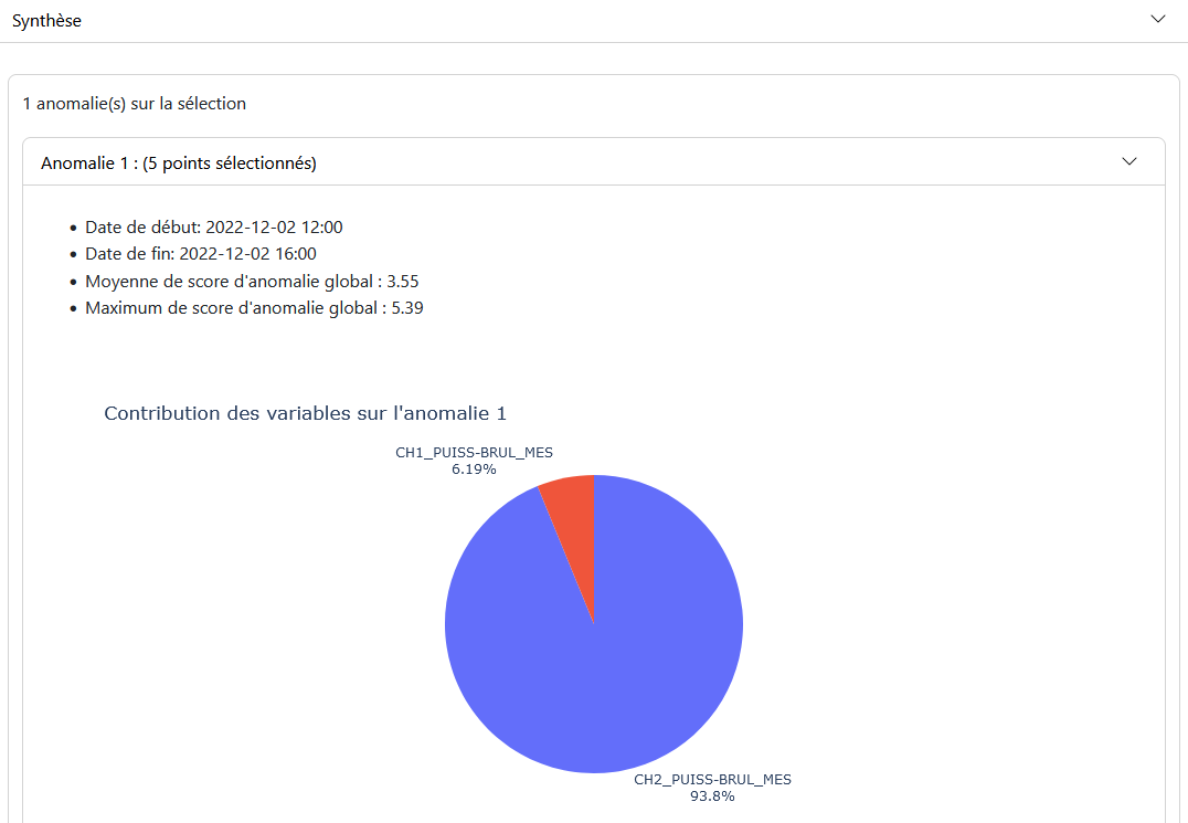
• Summary Panel: Provides a description of the anomalies over the given period and the contribution of the modeled variables to these anomalies.

“Historical” Tab

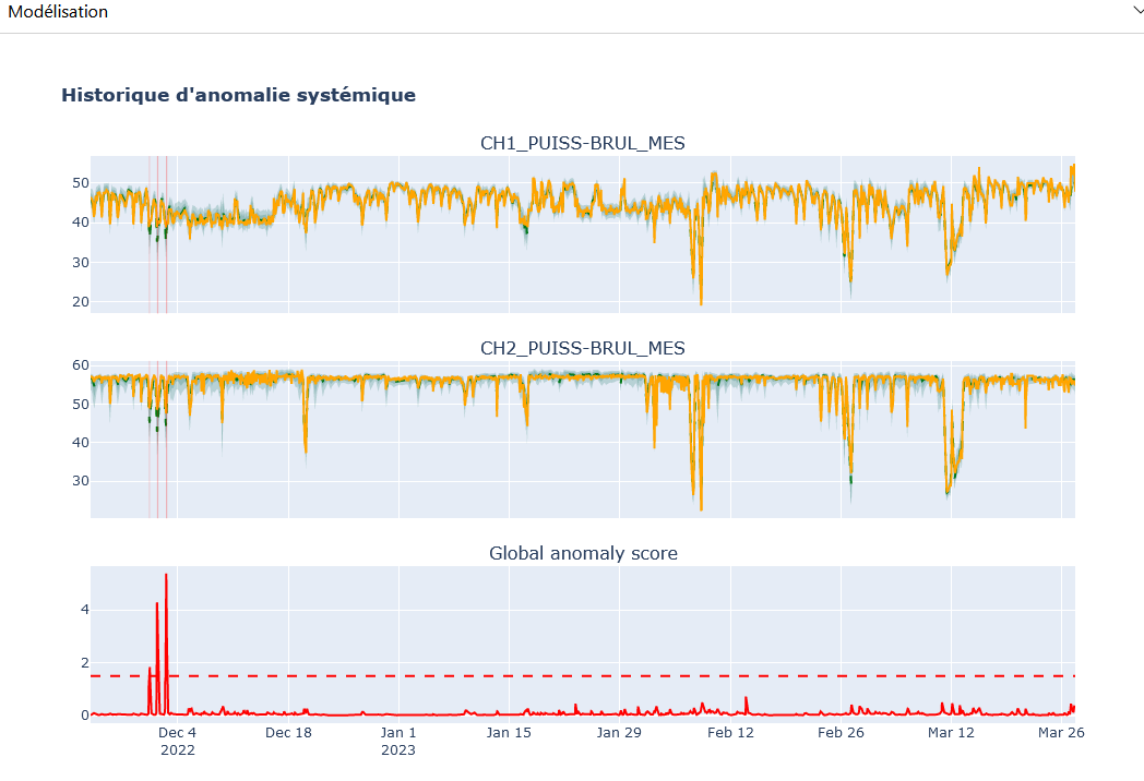
In the “Historical” tab, you will also find the configuration panels “System,” modeling “Modeling,” and summary “Summary.”

• Configuration Panel: Similar to the “Real-time” tab with the same choices. Allows you to choose the model, modeled variables, and displayed variables. Unlike the “Real-time” mode, there is no period selection, as the analysis covers the entire period of available data.

• Modeling Panel: Displays results based on the selected parameters. The user can select a specific period by clicking and holding on the obtained model.

• Summary Panel: Displays the results of anomalies for the selected period, with descriptions of the anomalies and the contribution of the modeled variables.

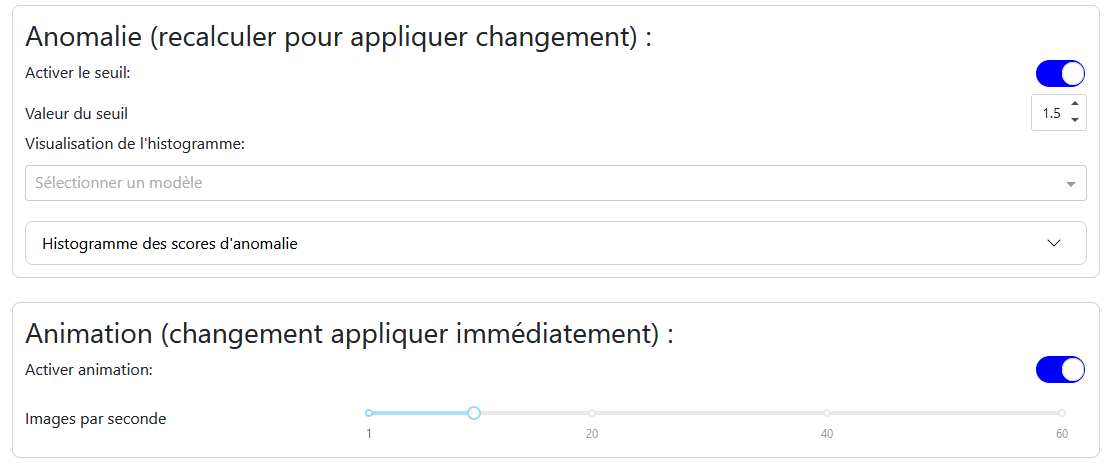
“Settings” Tab

• Anomaly: Allows you to enable the anomaly threshold and set its value. A histogram of anomaly scores helps determine the optimal threshold value.

• Animation: Allows you to enable or disable the animation and choose the number of frames per second.

3.3 - Impact Study

This feature allows for visualizing the impact of a variable, that is, the influences of variables on each other. It thus enables observing the consequences of modifying one or more variables on the others.

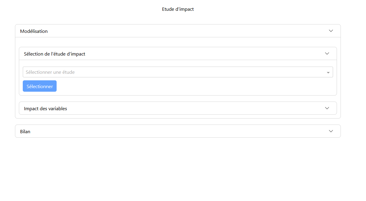
The interface consists solely of the “Impact Study” tab with the “Modeling” and “Summary” panels. In the “Modeling” panel, you will find the sub-panels “Impact Study Selection” and “Variable Impact.”

Selection Panel

In the selection panel, the user chooses the desired impact study. Once the study is selected, the modeling is displayed in the modeling panel.

Modeling Panel

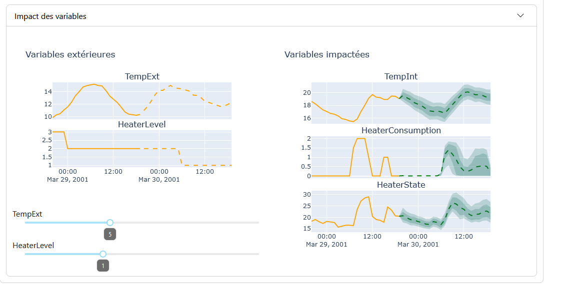
The modeling of the impact study is presented in two parts:

• External Variables: These are the hypothesis variables that influence the impacted variables. They are adjusted via sliders.
• Impacted Variables: These are the variables that change based on the external/hypothesis variables.

With each modification of the values of the external variables, the graphs of the impacted variables are regenerated. The modeling graphs are similar to those of the “Forecast Modeling” feature, with a few differences: for the graphs of the hypothesis variables, the part of the graph with prediction and uncertainty is replaced by a section representing the values set by the sliders.

Summary Panel

In the summary panel, different graphs are displayed depending on the chosen study. These graphs highlight the links and impacts between the variables. When the slider values are modified, the results of the graphs change accordingly.

Comparison with Other Features

Unlike other features, there are fewer options available (no selection choices for date/period or variables). In the context of a demo web app, these choices are determined by the study’s parameter file.

3.4 - Update, QOL ("Qualities Of Life")

Update

The update feature allows for adding and updating available models, configuration files, datasets, and default value files.

Tabs

There are three main tabs:

1. Models: Allows for updating, adding, and deleting models, as well as impact studies.
2. Datasets: Allows for updating, adding, and deleting datasets.
3. Preconfiguration: Allows for modifying the default values of models for their applications.

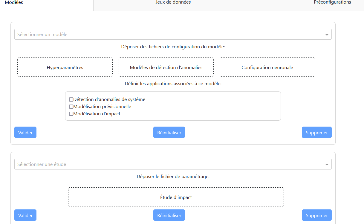
“Models” Tab

• Main Panel:

  • A dropdown menu to select the model.
  • An area to drop the necessary files (model, hyperparameters, neural configuration).
  • A checklist to select the applications associated with the model.
  • Three buttons: validation, reset, and deletion.

• Updating a Model:

  1. Select the model to update from the dropdown menu.
  2. Drop the new configuration files.
  3. Select the associated applications.
  4. Confirm with the “Validate” button.

• Adding a Model:

  1. Select “New Model” from the dropdown menu.
  2. Drop the necessary files.
  3. Select the associated applications.
  4. Confirm with the “Validate” button.

• Deleting a Model:

  1. Select the model to delete.
  2. Confirm with the “Delete” button.
  3. A dialog box will ask for confirmation.

• Impact Study:

  • A dropdown menu to select the study.
  • An area to drop the configuration file.
  • Three buttons: validation, reset, and deletion.

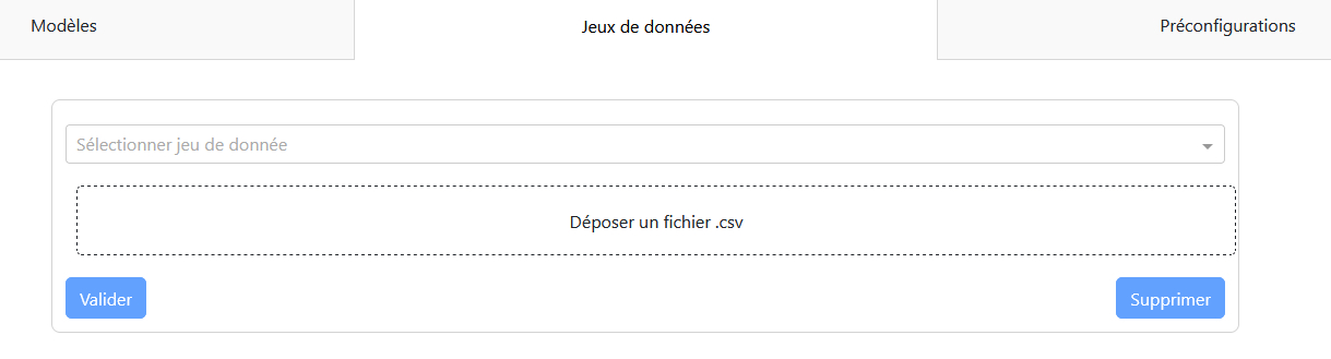
“Datasets” Tab

• Configuration Panel:

  • A dropdown menu to select the dataset.
  • An area to drop the data file.
  • Two buttons: validation and deletion.

• Modifying/Adding a Dataset:

  1. Select the dataset to modify or “New Dataset.”
  2. Drop the data file.
  3. Confirm with the “Validate” button.

• Deleting a Dataset:

  1. Select the dataset to delete.
  2. Confirm with the “Delete” button.

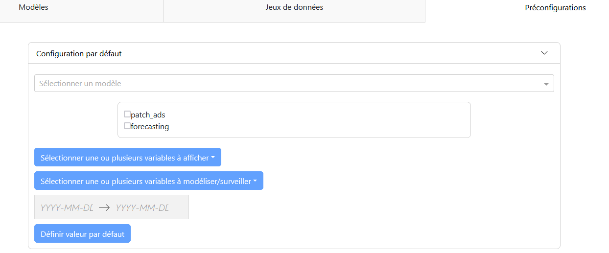
“Preconfiguration” Tab

• Configuration Panel:

  • A dropdown menu to select the model.
  • A checklist to select the application case.
  • Selection of variables to display and model.
  • Selection of the study period.
  • A validation button “Set Default Value.”

• Configuring Default Values:

  1. Select the model and application case.
  2. Configure the modeling parameters (displayed variables, modeled variables, period).
  3. Confirm with the “Set Default Value” button.

File Types

• Models: .tpkl files for models and .json files for hyperparameters.
• Impact Studies: Python file with configurations for the study.
• Datasets: .csv files containing the information used by models for predictions.
• Preconfigurations: .json file with values associated with models and the functionality used.